This post was inspired by an assignment submitted in the course Optimization by Yiftach Neumann and me.
In the first part, we described common optimization concerns in machine learning and introduced three widely used optimization methods: Momentum, RMSProp, and ADAM.
In this second (and last) part, we implement the aforementioned algorithms, show simulations, and compare them.
Algorithms, Implementations, and Evaluation
We provide implementation of the aforementioned algorithms in the python notebook:
Evaluation
on the optimizer behaviour
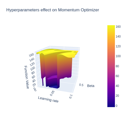
We can evaluate our algorithms by observing how well they perform optimization on various functions. Optimizers usually have hyper-parameters, such as learning rate, which have a dramatic effect on optimizer behaviour, as clearly seen in the figure to the right.
For this reason, in our work we compare optimizers after tuning their hyper-parameters. We performed an exhaustive search of ~50 different values for each parameter and chose the parameters that yielded the best value in the smallest number of iterations. The search was computationally expensive and might not be feasible over large datasets, so the results shown might be better than those seen in practice. Still, this is the best comparison method available to give each optimizer a fair try.
Low Dimensional Functions
We implemented three simple and complex functions over \(\mathbb{R}\) or \(\mathbb{R}^{2}\):
- Cubic Function \(\left(x^{2}\right)\)
- “Mean Squared Error” \(\left(x-y\right)^{2}\)
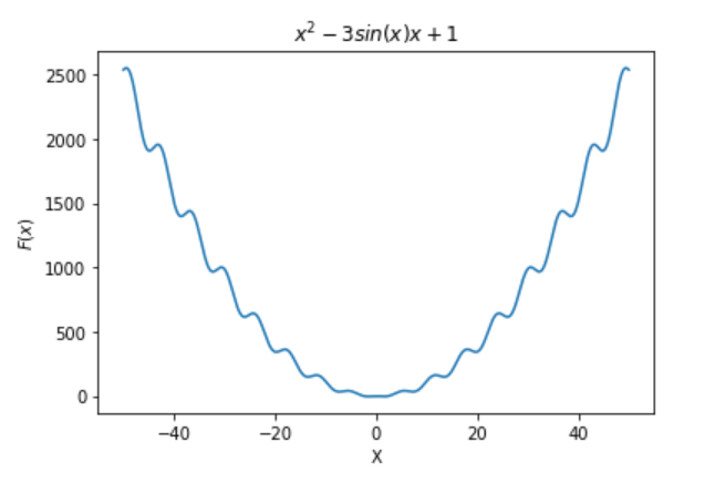
- “Hard Polynomial” \(\left(x^{2}-3\sin\left(x\right)x+1\right)\) (see figure to the right)
We then ran every optimizer on each of these functions, starting at different initial points. As mentioned before, all optimizers’ hyper-parameters were tuned. The results are detailed in Appendix A.
The results were quite surprising:
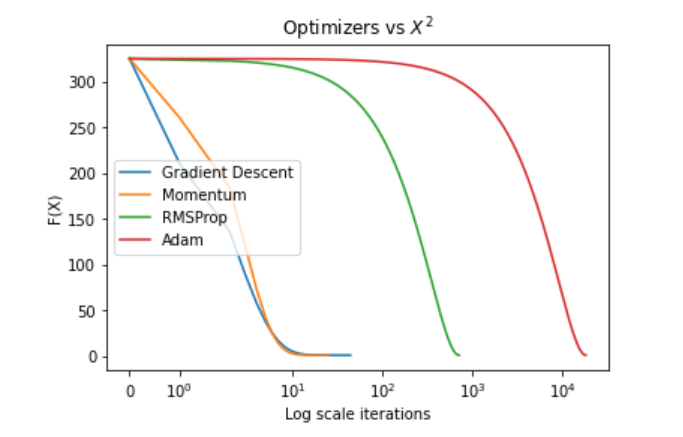
- On the simpler functions (Cubic and MSE), all of the optimizers converged to the global minimum.
- RMSProp and ADAM found an insignificantly lower spot, albeit at the price of a much larger number of iterations.
- Thus, on simple convex functions, Gradient Descent and Momentum will converge faster, without loss in performance.
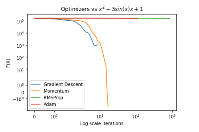
On the more challenging function, “Hard Polynomial”:
- There was a clear advantage to Momentum.
- On simple initial points (e.g., \(f\left(2\right)\)), all optimizers reached the global minimum.
- On points farther up the slope (e.g., \(f\left(401\right)\)), Momentum was the only algorithm that consistently converged to the global minimum with a reasonable number of iterations.
- Gradient Descent, with proper choice of learning rate, performed nicely as well for most initial points.
It is also clear that near the minimum point, ADAM and RMSProp converge slowly—a behaviour that was consistent in all functions and initial points, highlighting the importance of learning rate decay methods.
High Dimensional Cubic Functions
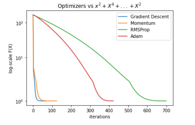
Next, we compared the optimizers on high-dimensional cubic functions, e.g., \(x_{1}^{2}+x_{2}^{4}+...+x_{n}^{2}\). These functions are interesting because one of the main motivations behind Momentum, RMSProp, and ADAM is to allow different changes in each dimension, in order to suppress oscillations in dimensions that have steeper slopes—allowing for fewer oscillations and better learning rate overall.
The results do not reflect the intuition:
- Gradient Descent had the lowest number of iterations by far, and ADAM consistently converged the slowest.
- With respect to performance, ADAM still converged to a lower point than the rest of the optimizers.
- Momentum had superior results to Gradient Descent, albeit with a small increase in iteration number.
- RMSProp performed the worst with a very large number of iterations.
For the full table of results, please refer to the appendix.
High Dimensional Polynomial
One of the main theoretical advantages of RMSProp and ADAM is the ability to choose a larger learning rate while reducing oscillations in dimensions with steeper slopes. We specifically chose these functions to highlight that behaviour. However, the plot above clearly shows that Momentum and Gradient Descent drop much faster towards the local minima, which raises questions about the correctness of this theoretical assumption. It is possible that ADAM’s popularity in the Deep Learning domain is due to another advantage that plays a role in the structure of loss function surfaces over the unique datasets of a particular deep learning domain.
High Dimensional Hard Polynomial
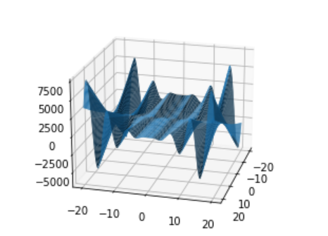
We implemented a function that is highly challenging for optimizers, as seen from the plot to the left:
The function is defined as \(x_{1}^{2}+x_{2}^{2}x_{1}\cos\left(x_{2}\right)+\ldots+x_{n}^{2}x_{1}cos(x_{n})+2n\). In many cases, the optimizers got lost in a “bottomless pit,” or missed a local minima and yielded very poor results.
Its shape over \(\mathbb{R}^{2}\) indicates how complicated this function is over higher dimensional domains. However, the hyper-parameter search proved itself and the optimizers dealt with the complexity, even in higher dimensions such as 5, 6, and 12.
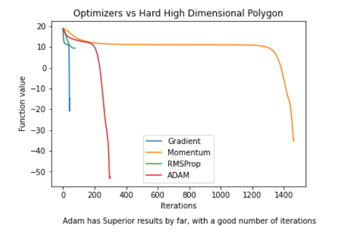
Hard High Dimensional Polynomial Plot
For all the initial points we checked, ADAM performed the best by a large margin and with a good number of iterations.
Conclusion
We implemented four optimizers that are highly popular within the Machine Learning community, and tested them on simple and complex functions, in order to test their performances in a sterile environment - perhaps simpler than the usual real data-set loss-function setting - and thus to gain insights about their behaviour.
It was clear that in simple convex functions, the simpler Gradient Descent and Momentum performed best. The theoretical ability of ADAM and RMSProp to use high learning rates while avoiding oscillations did not come into effect even in a setting that was supposed to give it a clear advantage. Yet, on a really complicated function, ADAM consistently performed best in terms of converging to a lower minima while keeping the number of iterations low. This suggests that ADAM performs best over complicated functions, which may explain why it is so successful in the Deep Learning real-practice domain. Our work also highlighted the importance of hyper-parameter tuning when using optimizers, and the importance of learning rate decay methods.
Bibliography
Adam Optimization Algorithm (C2W2L08)
How to implement an Adam Optimizer from Scratch
Introduction to optimizers
An Overview of Machine Learning Optimization Techniques
A Survey of Optimization Methods from a Machine Learning Perspective
Python notebook of gradient descent
ADAM: A METHOD FOR STOCHASTIC OPTIMIZATION
Barzilai, Jonathan; Borwein, Jonathan M. (1988). Two-Point Step Size Gradient Methods. IMA Journal of Numerical Analysis. 8 (1): 141. doi:10.1093/imanum/8.1.141.
Fletcher, R. (2005). On the BarzilaiBorwein Method. In Qi, L.; Teo, K.; Yang, X. (eds.). Optimization and Control with Applications. Applied Optimization. Vol. 96. Boston: Springer. pp. 235. ISBN 0-387-24254-6.